Fitting An Exponential Regression To Google Citation Data
In this post, I show how the scholar library can be used to explore historical citation data archived on Google Scholar in R. Using the scholar library, we import citation-related data, beginning in the year 1982, for two of the most important physicists of the 20th century – Stephen Hawking and Richard Feynman – and examine how their total citations evolved over time. For added fun, we fit a non-linear, exponential regression model to model their respective trends of citations over time.
First, we load the scholar library, locate the identification numbers for Hawking and Feynman (the identification numbers for authors on Google Scholar can be located in the URL for the author’s Google Scholar page), and use the compare_scholar_careers() function to import citation data for Hawking and Feynman beginning in the year 1982 and up to the most recent year.
library(scholar)
library(tidyverse)


#  Richard Feynman's and Stephen Hawking's IDs
ids <- c("B7vSqZsAAAAJ", "qj74uXkAAAAJ")

# Import Google Scholar data
df <- compare_scholar_careers(ids)


head(df)
            id year cites career_year            name
1 B7vSqZsAAAAJ 1982   581           0 Richard Feynman
2 B7vSqZsAAAAJ 1983   605           1 Richard Feynman
3 B7vSqZsAAAAJ 1984   657           2 Richard Feynman
4 B7vSqZsAAAAJ 1985   644           3 Richard Feynman
5 B7vSqZsAAAAJ 1986   726           4 Richard Feynman
6 B7vSqZsAAAAJ 1987   718           5 Richard Feynman
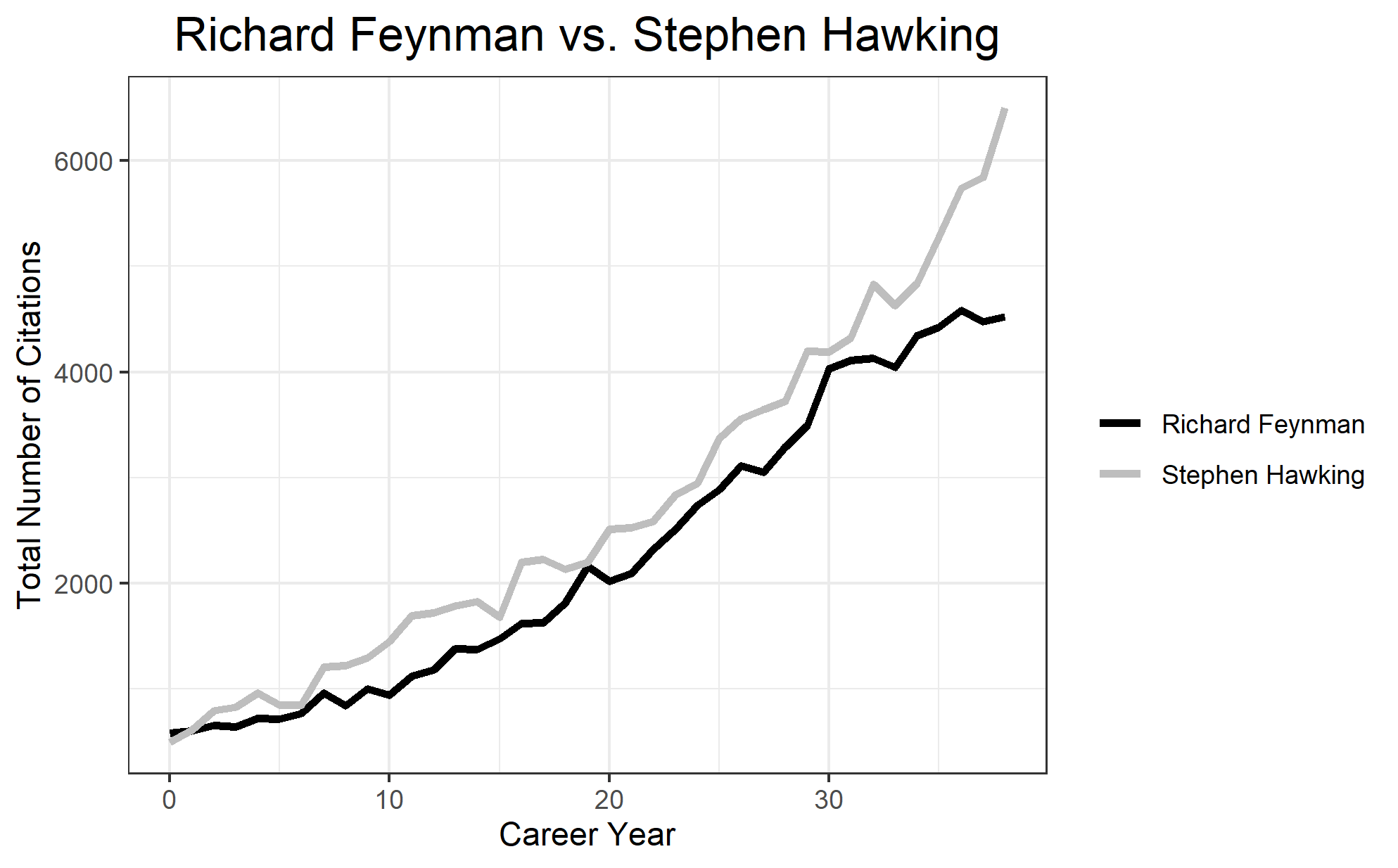
Plotting the total number of citations since 1982 (here we use the career_year variable generated by compare_scholar_careers(), which standardizes the year 1982 as the start of the career), we observe a positive trend in citations that appears to rise in an exponential manner. Moreover, at least from 1982, Hawking appears to eclipse Feynman in terms of absolute number of total citations.
Modelling Stephen Hawking’s and Richard Feynman’s Citation History
From plotting the data, the total citations from Hawking and Feynman both appear to follow an exponential trend over the course of their citation history. We can try fitting a non-linear regression model for each author, specifically estimating parameters for an exponential model of the form:
where y-prime is the predicted number of citations since the career start, x is the number of years since career start (x = 0 would reflect the year 1982 in this example), and alpha and beta are parameters to be estimated.
We use the nls() in R for fitting non-linear models via a non-linear least-squares method, where we can specify the above formula for an exponential model and supply initial parameters for alpha and beta for the optimization procedure. To derive initial parameters, we, first, fit a simple linear regression model on the citation data using log-transformed citation data. (If the trend is truly exponential, log-transforming the dependent variable should yield a linear relationship between log(y) and x.) We, then, save the coefficients of this model and use them as starting parameters in the initial instantiation of our nls() model. Finally, we plot the predicted values of the exponential model against the citation data from Google Scholar to visually examine the fit of the model against the empirical data.
# Fit exponential model to Feynman

df.feynman <- df %>%
  mutate(cites.log = log(cites)) %>% # log transform cites for simple linear regression
  filter(name == "Richard Feynman") %>%
  filter(career_year != max(career_year)) # remove latest year


m.lm <- lm(cites.log ~ career_year, data = df.feynman) # linear regression to get starting coefficients
st <- list(a = exp(coef(m.lm )[1]), b = coef(m.lm )[2]) # intercept (remember to take exp()) and slope coefficients
m.exp <- nls(cites ~ I(a*exp(b*career_year)), data=df.feynman, start=st, trace=T) # non-linear regression with least squares

m.exp.fitted <-fitted(m.exp) # save fitted values

# Summary
summary(m.exp)

Formula: cites ~ I(a * exp(b * career_year))

Parameters:
   Estimate Std. Error t value Pr(>|t|)
a 7.194e+02  4.138e+01   17.39   <2e-16 ***
b 5.217e-02  1.876e-03   27.81   <2e-16 ***
---
Signif. codes:  0 '***' 0.001 '**' 0.01 '*' 0.05 '.' 0.1 ' ' 1

Residual standard error: 248.5 on 37 degrees of freedom

Number of iterations to convergence: 5
Achieved convergence tolerance: 7.981e-06


# coefficients
coef(m.exp)
           a            b
719.37917740   0.05217138
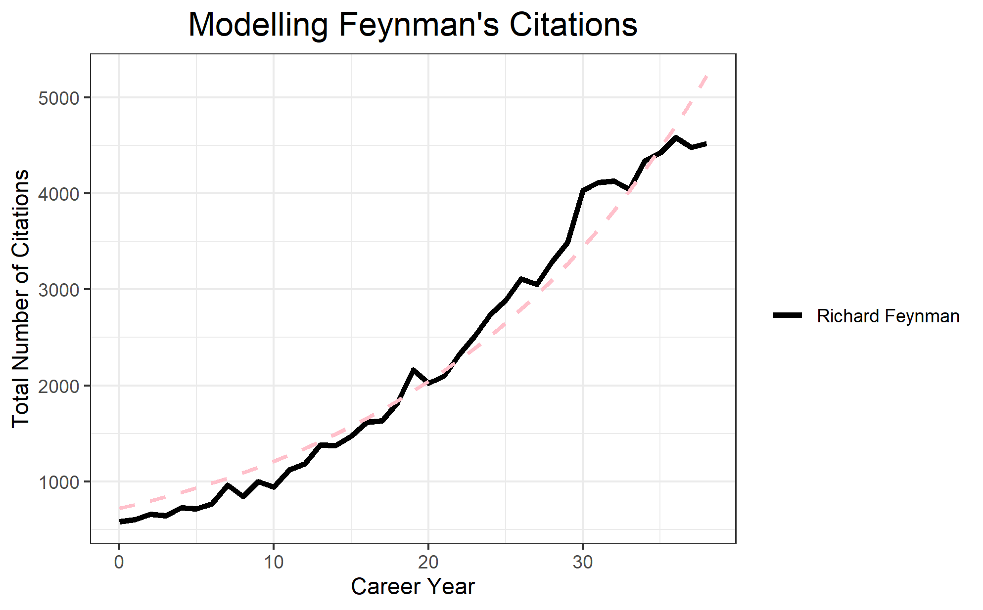
The parameters of the estimated exponential model were found to be significant, suggesting that an exponential model of the following form captures the trend observed in Feynman’s citation data beginning in 1982:
Visualizing the data against the model prediction, we find that the predicted values from model, denoted by the pink dashed line, seems to capture most of the the exponential trend, albeit the tails of the trend.
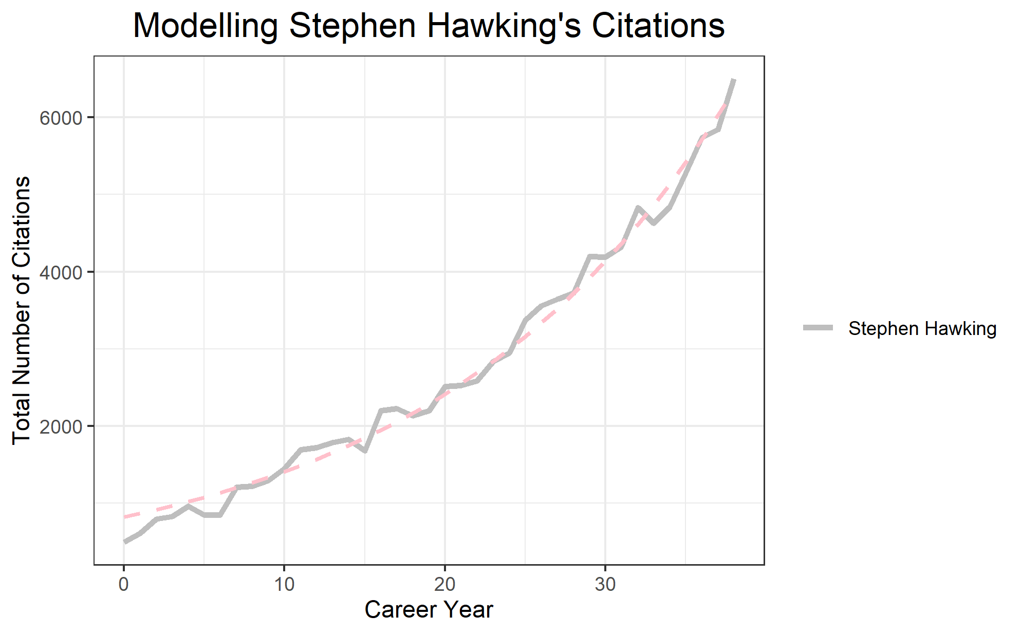
Repeating the same procedure to model the Hawking data, we get:
# Fit exponential model to Hawking


df.hawking <- df %>%
  mutate(cites.log = log(cites)) %>% # log transform cites for simple linear regression
  filter(name == "Stephen Hawking") %>%
  filter(career_year != max(career_year)) # remove latest year


m.lm <- lm(cites.log ~ career_year, data = df.hawking) # linear regression to get starting coefficients
st <- list(a = exp(coef(m.lm)[1]), b = coef(m.lm)[2]) # intercept (remember to take exp()) and slope coefficients
m.exp <- nls(cites ~ I(a*exp(b*career_year)), data=df.hawking, start=st, trace=T) # non-linear regression with least squares

m.exp.fitted <-fitted(m.exp) # save fitted values

# Summary
summary(m.exp)


Formula: cites ~ I(a * exp(b * career_year))

Parameters:
   Estimate Std. Error t value Pr(>|t|)
a 8.240e+02  2.725e+01   30.24   <2e-16 ***
b 5.379e-02  1.073e-03   50.15   <2e-16 ***
---
Signif. codes:  0 '***' 0.001 '**' 0.01 '*' 0.05 '.' 0.1 ' ' 1

Residual standard error: 167.9 on 37 degrees of freedom

Number of iterations to convergence: 4
Achieved convergence tolerance: 7.586e-07


# Coefficients
           a            b
823.96882888   0.05378992
Similar to the Feynman model, the estimated parameters for the Hawking model were also significant, yielding an exponential model with the following parameters:
Visualizing the data against the model prediction, we find that the Hawking model, again, denoted by the pink dashed line, captures the exponential trend quite well.