Dynamical Systems Models of Adaptive-Frequency Oscillators
Non-linear oscillators have become widely adopted in cognitive science as models of synchronization and entrainment—a dynamic process in which a system’s activity aligns in time with an external, time-varying input signal. Indeed, many systems that are of interest to cognitive scientists, across multiple scales of organization, exhibit a remarkable ability to synchronize their behavior to time-varying signals, such as the synchronized activity of neural ensembles to sensory stimulation, synchronized human action to auditory rhythms (e.g., music), and the macro-scopic synchronized activity of large social groups, such as fireflies and drum circles. Models of oscillation are particularly suited to explain these kinds of synchronized phenomena, as they possess all kinds of synchronization dynamics, such as phase-, mode-, and frequency-locking, that emerge naturally from dynamical laws that govern their motion and their coupling to input signals. Such oscillatory dynamics may reflect the physical principles that underlie how neural systems, agents, and social groups coordinate their activity over time.
There are cases, however, in which an oscillator might fail to synchronize to an input signal. One case is when the frequency of an input signal falls outside the entrainment basin of an oscillator, prohibiting the oscillator to enter a synchronized state with the input signal. In a 2006 paper, Righetti, Buchli, & Ijspeert (2006) proposed a Hebbian learning rule for several classes of oscillator models that allows an oscillator to learn the frequency of an external input signal, even for input frequencies that would normally fall outside the entrainment basin of a fixed-frequency oscillator. When equipped with the learning rule, an oscillator will adjust its natural frequency to a target frequency component reflected in an external input signal. In the case of sinusoidal forcing, the adaptive-frequency oscillator will tune its natural frequency to the fundamental frequency (F0) of the input. If the input signal is more complex—i.e., it contains multiple constituent frequencies—then the learning rule enables the oscillator to synchronize to one of input signal’s frequency components, depending on the initial natural frequency of the oscillator. Furthermore, if the oscillator itself contains multiple frequency components (e.g., a relaxation oscillator), then the learning rule will tune one of the oscillator’s frequency components to a frequency in the input signal.
Recently, I began to implement Righetti, Buchli, & Ijspeert (2006)’s Hebbian learning rule in MATLAB for several classes of oscillators analyzed in their manuscript: the Hopf oscillator, the Van der Pol oscillator, the Rayleigh oscillator, the Fitzhugh-Nagumo oscillator, and the Rossler strange attractor. You can track my progress by downloading my code on my github page. In this post, I share some initial simulations of the Hebbian learning rule with the first of the oscillator models presented in the manuscript—the Hopf oscillator.
Simulations Of An Adaptive-Frequency Hopf Oscillator
The Hopf oscillator is a non-linear oscillator that spontaneously oscillates, i.e., spontaneously enters a limit cycle, producing a non-zero amplitude. The equations of motion for the Hopf oscillator are given by the following system of ODEs, here represented in Cartesian coordinates:
Where r = sqrt(x^2 + y^2), mu > 0, F is the input signal, omega is oscillator natural frequency, and epsilon is a coupling coefficient to the input signal (and the learning rate; see below). Righetti et al., (2006) introduces a Hebbian learning rule for the Hopf oscillator that takes the following form:
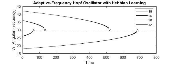
The learning rule governs the dynamics of omega, which is the control parameter for oscillator natural frequency in the Hopf oscillator. F, again, is the input signal, and epsilon controls the learning rate of the system. Below, I run several numerical simulations of a Hopf oscillator with adaptive-frequency dynamics to qualitatively assess the learning dynamics of the Hebbian learning rule. We start by simulating the frequency adaption of the Hopf oscillator for several initial conditions of the oscillator’s natural frequency (omega_0) to observe whether the oscillator correctly “learns” the frequency of the external input signal. In this simulation, a Hopf oscillator is being driven by periodic forcing at 30 Hz. Examining the dynamics of oscillator frequency for several initial conditions (omega_0 = 18, 26, 36, 40 Hz), we find that, for all initial conditions, the frequency of the oscillator converges to the frequency of the external input signal—30 Hz. (Moreover, for all initial conditions, there is a momentary increase in the variability of oscillator frequency right before the oscillator synchronizes to the external signal at its learned frequency.)
In the time domain, we can also clearly identify the moment when an oscillator learns the frequency of the input signal and enters a phase-locked relationship with the input signal. Let’s run a similar simulation with a slower input signal of 3 Hz, as we can more readily observe the dynamics of frequency adaptation in the time. With an initial condition of omega_0 = 10 Hz, we observe that an initial 10-Hz Hopf oscillator successfully “learns” the frequency of the 3-Hz input signal, as evinced by the dynamics of the oscillator’s natural frequency (i.e., omega). This learning is also evident in the time domain: as the Hopf oscillator nears the moment of synchronization (time 120 - 140), the phase of the oscillator fluctuates wildly before settling in lock-step with the driving signal. (The gif below shows the simulation from time 120 – 140, right before and after the oscillator learns the frequency of the input signal.)
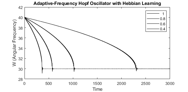
Next, we can investigate the effect of the learning rate, the epsilon parameter, on the dynamics of frequency adaptation. I aimed to replicate Figure 2 from the manuscript, which reports the effect of increasing the learning rate on the dynamics of frequency adaption. Similar to our first simulation, the oscillator is being driven by periodic forcing at 30 Hz, but now we vary the epsilon parameter, which controls the learning rate of the system. The initial condition of oscillator natural frequency is set to 40 Hz for several learning rates. Unsurprisingly, a slower learning rate requires more time for the oscillator to learn the frequency of the external signal (epsilon = 1 converges < 500 time, while epsilon = 0.4 converges > 2000 time). However, it is clear that the learning rate controls the overall timescale of frequency adaption.
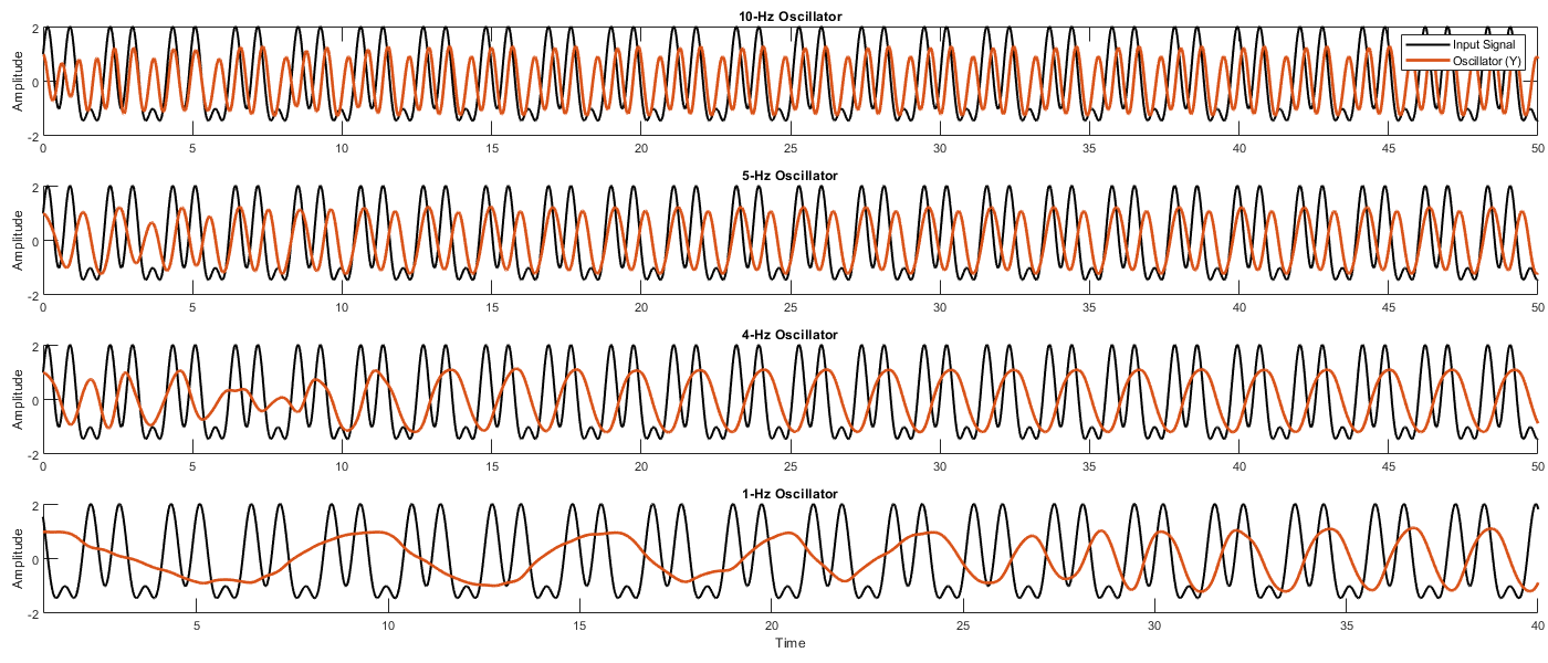
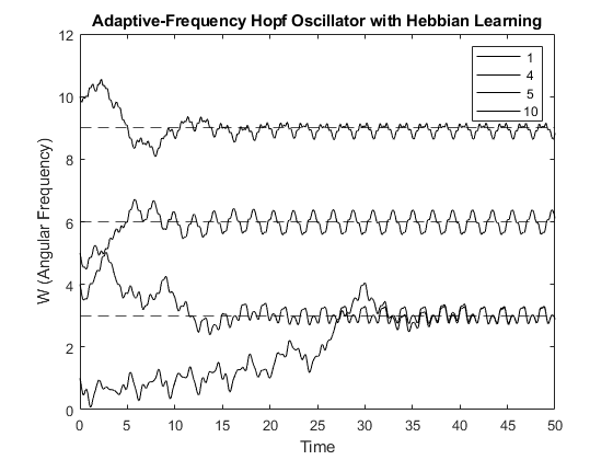
Finally, I explored whether an adaptive-frequency Hopf oscillator can learn the frequency content of a complex input signal. First, we create a complex signal containing multiple frequencies; in this example, a complex waveform containing a fundamental frequency of 3 Hz (F0) and two harmonics at 6 Hz (F1) and 9 Hz (F2). We simulate the model for the initial conditions, omego_0 = 1, 4, 5, 10 Hz. Plotting omega over time for each initial condition, we see that the 1-Hz oscillator learns the 3-Hz component of the input signal. This is also the result for the 4 Hz oscillator. (Interestingly though, the 4-Hz oscillator starts to increase in frequency during the beginning of the simulation until it tunes its natural frequency to ~ 5 Hz, then it slows down, heading towards the 3 Hz component of the input signal). The 5-Hz oscillator learns the 6-Hz component, and the 10-Hz oscillator learns the 9-Hz component.
In the time domain, we can clearly see how the oscillators align with the events in the complex waveform. For instance, after learning the new frequency, the 1-Hz oscillator phase-locks to the second high-amplitude event; the 4-Hz oscillator also phase-locks to the second high-amplitude event; the 5-Hz oscillator phase locks to both high-amplitude events; and the 10-Hz oscillator phase-locks to the all the events (e.g., those low-amplitude peaks and the high-amplitude peaks).